Sample Size Calculator: How Many Visitors for Valid A/B Tests?
A sample size calculator answers the most consequential question in conversion testing: how many visitors do you need before the result of an A/B test is statistically trustworthy? Stop too early and the winner you celebrate is often noise. Run too long and you burn traffic that could have funded the next experiment. The math behind the calculator is settled — yet most teams still launch tests without ever doing it.
This guide walks through the four inputs that determine sample size, explains why minimum detectable effect is the only one you genuinely control, and shows three worked scenarios for low-, medium-, and high-traffic sites. The closing checklist mirrors what statisticians at Microsoft, Booking, and Optimizely consider non-negotiable before a test goes live.
Why Sample Size Matters
An underpowered test hides real wins. With too few visitors, the natural variance of conversion data swamps the actual treatment effect, and the test concludes “no significant difference” even when a meaningful improvement exists. Specifically, this is a false negative — a Type II error — and the consequence is that good ideas die quietly without ever shipping.
Conversely, an overpowered test wastes traffic. If your test is configured to detect a 1% lift but the real effect is 15%, you have spent weeks of traffic to confirm what you could have proven in days. That cost is real because traffic is finite. Each week one variant runs is a week another idea cannot be tested.
The mathematics that connect these two extremes are not optional. Furthermore, they apply whether you call your method “frequentist statistics,” “null-hypothesis significance testing,” or simply “an A/B test.” The sample size calculator translates those equations into a single number: the visitors per variant required for a given level of certainty.
The 2018 Microsoft analysis of Bing’s experimentation platform reported that more than 80% of ideas tested by their teams did not move the target metric. In short, most experiments fail — and detecting the few real wins demands disciplined sample sizing.
The Four Inputs to Sample Size: Baseline Conversion Rate, MDE, Significance Level, Power
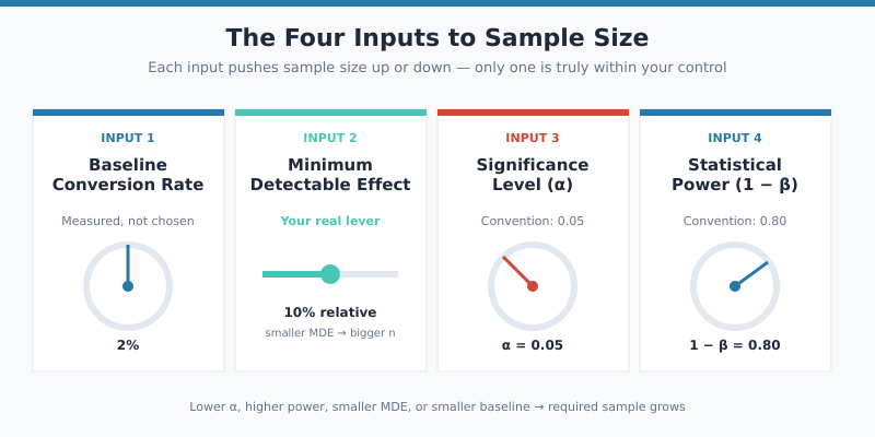
Every sample size calculator — from Evan Miller’s classic page to the engines built into Optimizely and VWO — uses the same four inputs. Understanding what each one represents is the difference between configuring a calculator thoughtfully and copying numbers without context.
- Baseline conversion rate — the historical performance of the page or flow you are testing. You measure this from analytics; you do not choose it.
- Minimum detectable effect (MDE) — the smallest improvement you care about detecting. This is your only true lever.
- Significance level (α) — the false-positive tolerance, conventionally 0.05.
- Statistical power (1 − β) — the probability of detecting a real effect if one exists, conventionally 0.80.
Two of these inputs are conventions held nearly universal across industry: α = 0.05 and power = 0.80. The remaining two — baseline rate and MDE — depend entirely on your business context. Therefore, sizing a test starts with measurement, not arithmetic.
Baseline Conversion Rate
Pull this from the past four full business cycles, not the past 30 days. A weekly cycle smooths weekday-vs-weekend variance; a monthly cycle smooths payday peaks; a quarterly cycle catches seasonality. Specifically, e-commerce baselines often differ by 30-40% between mid-month and end-of-month windows, and using a stale or atypical baseline corrupts every downstream calculation.
The Three Other Inputs
Power and significance are conventions you should rarely deviate from. MDE, by contrast, is a strategic decision the team needs to make before opening the calculator — and the next section explains why.
Minimum Detectable Effect (MDE): The Lever You Actually Control
MDE is the smallest improvement that would change your decision. If your CTA copy test only moves conversion from 5.0% to 5.05%, would you ship it? Probably not — the engineering effort, the QA cost, and the reduced ability to launch other tests on the same page make a 1% relative lift uneconomic. So 1% is not your MDE. It is below your decision threshold.
Your MDE is the lift size where shipping becomes obviously worthwhile. For most B2B SaaS landing pages, that floor sits around 10-15% relative. For high-volume e-commerce checkouts, where each conversion-rate point translates to seven-figure revenue, MDE drops to 2-5%. Furthermore, the smaller your MDE, the larger your required sample.
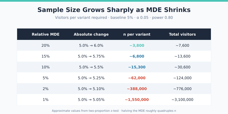
Notice the curve: halving the MDE roughly quadruples the required sample size. Going from 10% MDE to 5% MDE is not “twice as hard” — it is four times as expensive in traffic. As a result, MDE is the parameter that turns a feasible 14-day test into an impossible 56-day test.
Practical heuristic: set MDE to the smallest lift that would survive your CFO asking “is this worth the engineering?” That number is rarely below 5% relative for most teams.
Relative vs Absolute MDE
“5% MDE” is ambiguous. A 5% absolute change at a 5% baseline is a doubling — a 100% relative lift. A 5% relative change at the same baseline is just 0.25 absolute percentage points. Calculators should specify which they use. In addition, almost all reputable tools default to relative MDE because it scales naturally across funnels with very different baseline rates.
Significance vs Power: What α=0.05 and 1−β=0.80 Really Mean
These two parameters control your tolerance for two different kinds of error. The table below summarises the trade-off cleanly.
| Term | Symbol | Convention | What it controls | What it costs |
|---|---|---|---|---|
| Significance level | α | 0.05 | False-positive rate (Type I error) | Lower α → larger sample |
| Power | 1 − β | 0.80 | True-positive rate (1 minus Type II error) | Higher power → larger sample |
| Confidence | 1 − α | 0.95 | Inverse of significance — how often confidence intervals contain the true effect | Same as α |
| False-negative rate | β | 0.20 | Probability of missing a real effect | Inverse of power |
α = 0.05 means you accept a 5% chance of declaring a winner when no real difference exists. Power = 0.80 means that if a real lift of MDE size does exist, you have an 80% chance of detecting it. Notice the asymmetry: industry treats false positives as four times more costly than false negatives. That convention dates back to Fisher and Neyman, and the Evan Miller sample size calculator bakes both defaults in.
When to Deviate from Defaults
For high-stakes decisions — pricing changes, fundamental UX rewrites, anything that touches revenue directly — bump power to 0.90 and tighten α to 0.01. The sample-size cost is steep, but a false positive on a pricing test can damage trust for quarters. Conversely, for low-risk copy tests, 0.05 and 0.80 are perfectly defensible and have been the industry standard since at least the early 2000s.
The Sample Size Formula (and Why You Don’t Calculate It by Hand)
For a two-sided test comparing two proportions with equal allocation, the textbook formula is:
n = (Zα/2 + Zβ)² · [p₁(1−p₁) + p₂(1−p₂)] / (p₁ − p₂)²
Where p₁ is the baseline rate, p₂ is the rate after applying the MDE, Zα/2 ≈ 1.96 for α=0.05, and Zβ ≈ 0.84 for power=0.80. The result n is the visitors per variant; total traffic required is 2n.
Plugging in a 5% baseline and 10% relative MDE (so p₂ = 5.5%): n ≈ 15,300 per variant. Doubling that gives the ~30,600 visitors total needed. In practice, software handles this — typing 5% and 10% into a calculator returns the answer in milliseconds, and modern tools also account for unequal allocation, sequential testing corrections, and continuity adjustments that the textbook formula ignores.
Use the A/B Test Calculator to verify significance after the test ends. For pre-test sizing specifically, Evan Miller’s calculator and the statsmodels NormalIndPower class in Python are the standards most analysts trust.
Why Hand Calculations Are a Trap
The textbook formula assumes equal allocation, two proportions, no adjustment for multiple comparisons, and a single endpoint. Real tests violate at least one of these assumptions almost always. Specifically, if you test five variants against a control, you need a Bonferroni correction; if you peek at results midway, you need an alpha-spending function; if your conversion is rare (under 1%), the normal approximation breaks and you need exact tests. Software handles these corrections; mental arithmetic does not.
Working Examples: Three Real Test Scenarios
The following three scenarios — drawn from common portfolio sites — show how MDE and traffic budget interact in practice.
| Scenario | Site type | Baseline | MDE | n per variant | Weekly traffic | Test duration |
|---|---|---|---|---|---|---|
| Low-traffic SaaS | B2B landing page | 3% | 20% relative | ~6,800 | 1,500 visitors | ~9 weeks (infeasible) |
| Mid-traffic blog | Newsletter signup | 8% | 15% relative | ~3,900 | 4,000 visitors | ~2 weeks |
| High-traffic e-commerce | Product page CTR | 12% | 5% relative | ~24,000 | 50,000 visitors | ~1 week |
Scenario 1: The Low-Traffic SaaS Trap
The 6,800 visitors per variant the calculator demands is achievable in absolute terms — but at 1,500 weekly visitors total (split 50/50, that’s 750 per variant per week), reaching n takes nearly 9 weeks. Most products cannot freeze a test for that long. The team’s options are to widen MDE to 30% (cuts n by half), focus on higher-traffic pages, or shift to qualitative methods like user interviews and session replay.
Scenario 2: The Sweet Spot
The mid-traffic blog can complete its test in 2 weeks at 15% MDE. As a result, this team can run roughly 25 well-powered experiments per year on a single page. That cadence is what compounds into measurable conversion gains over time.
Scenario 3: The Luxury of Volume
The e-commerce site can detect a 5% relative lift on CTR within a week. With that traffic, the team can also afford tighter significance thresholds (α=0.01) and higher power (0.90) without blowing the runtime budget. High-traffic sites are not “easier” to optimise — they are easier to measure, which is what makes their optimisation programmes so productive.
One-Tailed vs Two-Tailed Tests (When Each Is Justified)
A two-tailed test asks “is the variant different from control, in either direction?” A one-tailed test asks “is the variant better than control?” The one-tailed version requires roughly 25% fewer visitors at the same α and power — which sounds tempting, until you understand the cost.
One-tailed tests forbid you from concluding the variant is worse, even if data shows clear damage. If your “improvement” actually drops conversion by 30%, a one-tailed test cannot detect that — it only declares either “winner” or “no significant difference.” Therefore, the variant is treated as a non-result and may even ship.
| Test type | Use when | Avoid when |
|---|---|---|
| Two-tailed | Default — virtually all conversion testing | Never — it is always defensible |
| One-tailed | Pre-registered hypothesis, no possibility of harm, one direction makes business sense | You are tempted by the smaller sample size — that is the wrong reason |
In short, default to two-tailed. VWO’s documentation and most experimentation platforms now make two-tailed the only option, precisely because the marginal sample-size saving is rarely worth the analytical risk.
Sequential Testing and Bayesian Alternatives
The classical sample size calculator assumes a fixed-horizon design: you compute n, run until you hit n, then check significance once. Two alternatives loosen this constraint, though both come with their own discipline requirements.
Sequential testing uses techniques like alpha-spending or always-valid p-values to allow legitimate peeking at the data as it accrues. Optimizely’s Stats Engine and similar platforms implement this. The benefit is that strong winners can stop early; the cost is roughly 10-30% larger total sample size when no early stop occurs.
Bayesian A/B testing reframes the question entirely. Instead of “is the difference significant at α=0.05?”, it asks “what is the probability that B beats A?” The calculation is conceptually different but the sample size requirements end up similar in practice. Booking.com, among others, has published extensively on running Bayesian platforms at scale.
For most teams, the classical fixed-horizon design with a sample-size calculator remains the simplest and most defensible approach. Furthermore, switching frameworks does not eliminate the need to plan sample size in advance — it just changes the formula.
Common Sample-Size Mistakes
The errors below appear in roughly that order of frequency across teams I have audited. Each one inflates false-positive rates above the nominal 5% — sometimes catastrophically.
- Peeking — checking results before n is reached and stopping when “significant.” This inflates Type I error to 30-50% in extreme cases. The fix is a pre-registered analysis date, or a sequential-testing platform that handles peeking correctly.
- Rebuilding ammunition — running the same test repeatedly until one finally “wins.” Each rerun is another shot at the 5% false-positive lottery. After 20 attempts, the cumulative false-positive rate exceeds 64%.
- Ignoring variance — the formula assumes binary conversion data. Revenue per visitor, AOV, and engagement metrics have much higher variance and need different calculators (often 5-10x larger samples).
- Confusing relative and absolute MDE — typing “5%” into a calculator that expects absolute when you meant relative produces wildly wrong sample sizes.
- Using a stale baseline — last quarter’s conversion rate may not match this quarter’s. Recompute every time.
- Underpowering on purpose — “we’ll just stop when we see something” is not a test design. It is data dredging dressed up as experimentation.
Microsoft’s experimentation team estimates that fixing peeking alone improves win-rate accuracy by a factor of two to three. Similarly, the discipline of pre-registering n, the analysis date, and the stopping rule eliminates most of the failure modes above.
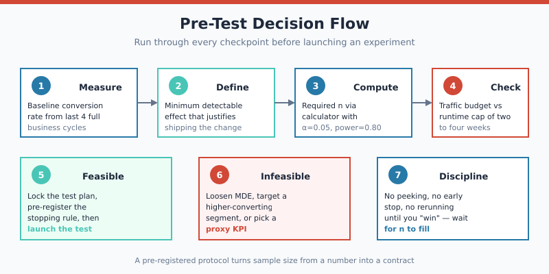
Pre-Test Checklist Before You Start
Run through every item below. If you cannot complete one, the test is not yet ready to launch.
- Baseline conversion rate measured from at least four full business cycles.
- MDE defined as the smallest lift that justifies shipping — not what you hope to find.
- Required n computed for α=0.05, power=0.80, two-tailed (override only with documented reason).
- Traffic budget verified — runtime under 4 weeks, ideally under 2.
- Stopping rule pre-registered — exact date or visitor count, not “when it looks significant.”
- Single primary metric declared — no fishing across 12 secondary metrics.
- Guardrail metrics identified — bounce rate, page load time, error rate (catches harmful variants).
- QA pass complete — both variants tested on mobile, desktop, all major browsers.
- Sample-ratio mismatch monitor active — flags broken randomisation early.
- Post-test analysis owner assigned before launch — not after results arrive.
For broader testing methodology, the A/B testing guide covers the full experimentation lifecycle. For interpreting results once the test ends, marketing ROI methods connect statistical wins to business impact.
From Calculator to Confidence
A sample size calculator is not a bureaucratic formality. It is the contract you sign with your data before you start collecting it. Specifying n, α, power, and the analysis date in advance turns A/B testing from opinion-laundering into evidence — and that is the only thing that compounds.
To compute the visitors required for your next test, run the inputs through the A/B Test Calculator. Combined with a disciplined pre-test checklist, that single number is the difference between experiments that move the business and experiments that merely fill dashboards.